Example 6.6.2: Solve , 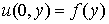using method of characteristics.

Solution: The characteristic equation is

      (but a=1, b=y)

 

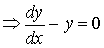
where C is a constant.

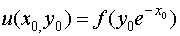
If the solution passes through (x₀, y₀) (that is x₀is a point on the initial curve) then which gives

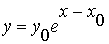
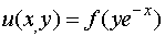
The solution along this characteristic is since the initial conditions are given at x=0 and each characteristic has to pass through the initial solution to have the given PDE a a unique solution we have . Hence the solution to the given PDE can be written as

or

General Theory of Characteristic Curves

The general theory of characteristic curves should encompass more general equations and not treat the variables x and y in an unsymmetrical way. Furthermore, the solution may not be constant along a characteristic curve; it may only satisfy ordinary differential equation along a characteristic.

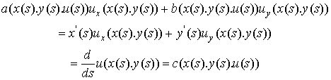
Consider the equation

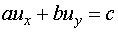
                                                                                                                 ................. (6.6.9)

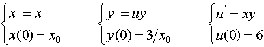
in which a, b and c are functions of x, y and u. Suppose that the value of the solution is known at a point (x₀, y₀). This could be the result of prior calculations or a boundary value that had been prescribed. We shall indiacate now how additional solution values of (6.6.9) can be obtained by integrating some ordinary differntial equations. Consider this system of three ordinary differential equations with initial conditions:

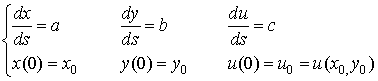
                                                                                                                  ................. (6.6.10)

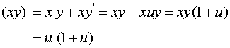
To produce a table of x(s), y(s), u(s) starting at s=0. One can integrate this system numerically. It is not hard to verify that this table will provide solution points of the partial diferential equation (6.6.9). Indeed.

(In this calculation primes indicate differentiation with respect to s)

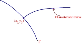
If the values of u(x,y) have been prescribed along some curve (not a characteristic curve) then in principle one can start at any point of , integrate system (6.6.10), and obtain additional values of u(x, y) along arcs. (See figure 6.6.1 for help in understanding this idea). The arcs obtained in this process are characteristic curves for Equation (6.6.9).

 

 

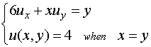
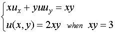
Example 6.6.3: Consider the partial differential equation

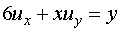
With u(3, 3) =4, what value of u(15, 21) is obtained by following a characteritic curve?

Solution

The characteristic curve through the initial point is governed by the initial-value problem

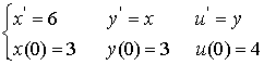
On integrating these equations, we obtain

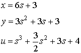
Letting s = 2, we arrive at x = 15, y = 21, u = 24.

Example 6.6.4: Use the method of characteristics to find a solution of the boundary-value problem

Solution : Let us find the characteristic curves passing through the point (x, y)=(r, r), r6.

We solve the system

'

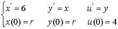and obtain

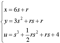
If (x, y) is a given point in the plane, we try to determine a corresponding (r, s) using the first two equations in (23). The result of this calculation is

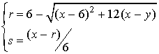
With the values of r and s at hand, the value of u at(x, y) can be computed from the third equation in (23). Thus for example, if (x,y)=(15,21), then (r,s)=(3,2) and u=24 as in Example 6.6.4.

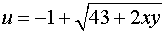
Example 6.6.5: Solve the boundary value problem

by the method of characteristics.

Solution: The equations for the characteristics are

Since

Integrating with respect to s given

but u(x, y) = 2xy when xy=3 given C=-21