Crank Nicolson method
If the forward difference approximation for time derivative in the one dimensional heat equation (6.4.1) is replaced with the backward difference and as usual central difference
approximation for space derivative term are used then equation (6.4.1) can be written as
.................
(6.4.4)
where i=1,2,3..........N-1 and n=1,2,3.................
or
.................
(6.4.5)
for i=1,2,3..........N-1 and n=0,1,2,3.................
.................
(6.4.6)
for i=1,2,3..........N-1 and n=0,1,2,3.................
since there are three unknown terms in each of the equations (6.4.6)
the scheme so obtained is an implicit method. The main drawback of having more
than one unknown coefficient in any equation, unlike FTCS method, is value of
the dependent variable at any typical node say (i, n) can't be obtained from
the single finite difference equation of the node (i, n) but one has to be generate
a system of equations for each time level separately by varying i. Then
for each time level there will be system of equations equivalent to the number of unknowns in that time level(say N-1 in the present case). This linear
system of algebriac equations in (N-1) unknowns has to be solved to obtain the solution for each time level . This process has to be repeated
until the desired time level is reached. The scheme(6.4.6) is called fully implicit
method.
Schemes (6.4.2) and (6.4.5) are two different methods
to solve the one dimensional heat equation (6.4.1). Crank-Nicolson scheme is then obtained by taking average of these two schemes that is
for i=1, 2, 3..........N-1 and n=0, 1, 2, 3.................
.................
(6.4.7)
for i=1, 2, 3..........N-1 and n=0, 1, 2, 3.................
Since more than one unknown is involved for each i in equation (6.4.7) Crank - Nicholson scheme is also an implicit scheme hence one has to solve a system of linear algebraic equations for every time level to get the field variable u.
The sketch for the Crank-Nicolson scheme is
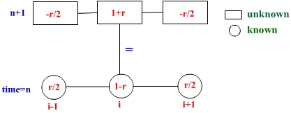
The linear algebraic system of equations generated in Crank-Nicolson method for any time level tn+1 are sparse because the finite difference equation obtained at any space node, say i and at time level tn+1 has only three unknown coefficients involving space nodes 'i-1' , 'i' and 'i+1' at tn+1 time level, so in matrix notation these equations can be written as AU=B , where U is the unknown vector of order N-1 at any time level tn+1 , B is the known vector of order N-1 which has the values of U at nth time level and A is the coefficient square matrix of order N-1 x N-1 with a tri-diagonal structure
A matrix of this structure that has only three non-zero terms at diagonal and one before and one after the principal diagonal for any row is called a tri-diagonal matrix and the system of equations with tridiagonal coefficient matrix is called tridiagonal system. Though direct solvers like Gauss elimination and LU decomposition can be used to solve these systems there are some special schemes available to solve the tridiogonal systems. One of them is Thomas algorithm which exploits the tridiogonal nature of the coefficient matrix. Thomas algorithm is similar
to Gauss elimination however, the novelty in the method is the forward elimination and back substitution parts of Gauss elimination are used only for the non-zero positions of the system AU=B.
Thomas Algorithm
Let us call the three non-zero diagonals of A as a, b and c where b
has the elements of the principal diagonal, a has the elements of the diagonal
before the principle diagonal with zero as the first element and c has the elements
of the diagonal which lie after the principal diagonal with a zero as the last
element then the order of a, b and c is equal to the number of unknowns for
any time level with the known vector B. Then the Thomas algorithm can
be written as
Do i=2 to N (if N is the number of unknowns)
end do

Do i = N-1 to 1

end do