In this method the time derivative term in the one-dimensional heat equation (6.4.1) is approximated with forward difference and space derivatives are approximated with second order central differences. This gives

            

        ................. (6.4.2)

where (i=0,1,2,3.......N.) and (n=0,1,2,3......). To distinguish between space and time coordinates superscript index n is used for time coordinate where as a subscript i is used to represent the space position as shown in the figure 6.4.1. N is the number of points on the length of the rod excluding zeroth point.

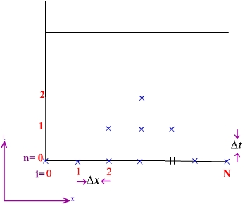
  Figure 6.4.1 Descritization of the domain

At any typical node(i, n) the finite difference equation can be written as

           

             ................. (6.4.3)

where gives a formula to compute the unknown temperature distribution on the rod at various positions at various times . For n=1, the unknown u is first calculated using the initial conditions at t=0 and boundary values at x=0 and x=L(where L is the length of the rod). Once the solution at time level 1 is obtained, the solution at n=2 is calculated in the same manner by making use of the solution at n=1 and the boundary conditions at x=0 and x=L. The same procedure is repeated until the solution reaches a steady state or until the required time level.

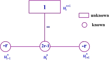
Since formula (6.4.3) has only one unknown for any i and n it is called an explicit scheme. The sketch for the FTCS scheme is

 

Example 6.4.1:

Find the temperature distribution on a uniform rod of length 1 unit at various times if the rod is kept at at the ends and has an initial distribution of the temperature x(1-x). (assume C=1).

Given      with C= 1

     boundary conditions and

    for 0 < x <1

let the step length in the space direction be 0.1       Analytical Solution

Case (i): r = 0.1       

Equation (6.4.3) reduces to

     i = 1,2,3.............9 and n = 0,1,2.............

The solution so obtained is given in the table 6.4.1 in the symmetric region.

i=	0	.1	.2	.3	.4	.5
n=0	0	.9	.16	.21	.24	.25
n=1	0	.088	.158	.208	.238	.248
n=2	0	.862	.156	.206	.236	.246
n=3	0	.846	.154	.204	.234	.244
……	……	……	……	……	……	……
n=10	0	.0757	.1413	.1902	.22	.23
……	……	……	……	……	……	……
n=20	0	.0669	.1262	.172	.2006	.2102
……	……	……	……	……	……	……
n=49	0	.0493	.0938	.1289	.1514	.1592

Table 6.4.1

Case (ii):

Equation (6.4.3) reduces to

and the solution for various i and various n is given in table 6.4.2.

i=	0	.1	.2	.3	.4	.5
n=0	0	.9	.16	.21	.24	.25
n=1	0	.08	.15	.2	.23	.24
n=2	0	.075	.14	.19	.22	.23
n=3	0	.07	.1325	.18	.21	.22
……	……	……	……	……	……	……
n=10	0	.0483	.0918	.1265	.1484	.1563
……	……	……	……	……	……	……
n=20	0	.0292	.0556	.0766	.899	.0946
……	……	……	……	……	……	……
n=49	0	.0068	.0130	.0178	.0210	.0221

Table 6.4.2

Case (iii)

Equation (6.4.3) reduces to

and the solution given in table 6.4.3

i=	0	.1	.2	.3	.4	.5
n=0	0	.9	.16	.21	.24	.25
n=1	0	.07	.14	.19	.22	.23
n=2	0	.07	.12	.17	.2	.21
n=3	0	.05	.12	.15	.18	.19
……	……	……	……	……	……	……
n=10	0	3.39	-5.44	6.11	-5.56	5.45
…….	……	……	……	……	……	……
n=20	0	.9303	-1.7483	2.3201	-2.3518	2.8796
……	……	……	……	……	……	……
n=49	0	-2.3636	4.4946	-6.1863	7.2724	-7.6467

Table 6.4.3

It is clear from tables 6.4.1, 6.4.2 and 6.4.3 that the solutions obtained with r=0.1 and r=0.5 are looking reasonable whereas the solution obtained with r=1 is unphysical because the temperature can't go to negative on the rod.

To investigate the accuracy of the scheme the numerical solution with r = 0.1, 0.5, 1.0 have been compared with analytical solution at time t = 0.1 (n=10 for r=1) for the symetric region of x that is between x=0 and x=0.5 in table no. 6.4.4 and the same has been given graphically in the figure 6.4.1.

x	0.0	0.1	0.2	0.3	0.4	0.5
Analytical	0	0.0297	0.0565	0.0778	0.0915	0.0962
r=0.1	0	0.029814	0.056708	0.07805	0.091751	0.096472
r=0.25	0	0.029594	0.056291	0.077478	0.091079	0.095766
r=0.5	0	0.029242	0.055552	0.076556	0.089884	0.094625
r=0.75	0	0.056235	-.8305	1.365	-1.38	1.605
r=1.0	0	3.39	-5.44	6.11	-5.56	5.46

Table 6.4.4

It is clear from the comparisons in table 6.4.4 and figure 6.4.1 that the error in the solution increases with r and become unphysical for r>0.5 (A theoretical justification is given in a later section). Hence to use FTCS scheme the computations have to be cariedout with r less than 0.5. Therefore for a given fixed step length in space direction say =0.1, the step length in time direction will become very small which leads to increase of number of iterations to reach the desired time level.