6.5 Elliptic Partial Differential Equations:
Mathematical modelling of steady state or equilibrium problems lead to elliptic partial differential equations. Equation (6.1.1) with the value of the descriminant  < 0 is the most general linear form of this type of PDE. These problems always occur as boundary value problems with partial differential equations valid in a region, say D with Dirichelt, Neumann or mixed boundary conditions prescribed on the boundary
  . The general form of these conditions are
1. Dirichelt condition:
................. (6.5.1)
2. Neumann condition
................. (6.5.2)
3. Mixed conditions
................. (6.5.3)
where a, b, f are some known functions, n is the normal direction, u is the dependent variable which has to be obtained by solving the PDE.
The best known elliptic Partial Differential Equations are Laplace's equation

................. (6.5.4)
where  in three-dimensional problems and the Poisson's equation

................. (6.5.5)
where f is some known function.
The elliptic PDE (6.5.4), (6.5.5) or (6.1.1) with < 0 with the neccessary boundary conditions (6.5.1), (6.5.2) or (6.5.3) can be solved numerically using finite difference methods in three steps.
In the first step the given domain D is superimposed with a finite difference mesh by identifying nodal points at which the given equation has to be solved to obtain the field variable. In the second step the partial derivatives in the differential equation and boundary conditions are approximated with finite difference coefficients resulting in a difference equation correspond to each nodal point of the domain D. In the third and last step the set of algebraic equations generated at the nodal points of the mesh have to be solved for the field variable using
either direct methods or iterative methods as explained in chapter 2.
Method of solution for Dirichlet Problem:
Consider the PDE

................. (6.5.6)
where A, B, C, D, E, F and G are some known functions satisfying <
0 and  on the domain D say
  . On the boundary of the domain assume Dirichlet boundary condition u=g, where g is a known function.
In the first step the square domain D: is descritised as
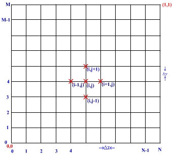
Figure 6.5.1 Descritisation of the square domain
By choosing grid points N+1 and M+1 in x-direction and y-directions respectively, the step lengths can be obtained as

................. (6.5.7)
and the coordinates of any typical node P(xi, yj) can be written as
where x0, y0 are the initial points respectively in x and y directions( (0,0) in the present case).
Since in the given Dirichtel problem the field variable u is known at i=0 and N and also at j=0 and M, it has to be obtained at i=1, 2, ....... N-1 and j=1, 2, .......M-1, that is totally at (N-1) * (M-1) nodal points.
The given PDE is approximated using finite difference coefficients at these nodal points to obtain (N-1)*(M-1) algebriac equations.
The corresponding finite difference approximation to (6.5.6) is
for i=1, 2, 3 . . .N-1 and j=1, 2, 3 . . . M-1

................. (6.5.8)
where
for i=1, 2, 3 . . .N-1, j=1, 2, 3 . . . M-1
The system of equations (6.5.8) can be written in the matrix form as

................. (6.5.9)
where u is the unknown and  is known column vector of order (N-1) * (M-1) and L is the square matrix of same order. Also due to the special nature of the equation (6.5.8) any row or column of L has only a maximum of 9 non-zero coefficients as shown in figure 6.5.2.
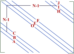
Figure 6.5.2 Structure of the coefficient matrix
The algebraic system (6.5.8) can be solved using either direct methods or iterative methods. However using iterative methods is a better choice to solve(6.5.8) compare to direct methods due to huge amount of storage required in using the former.
If the mathematical model of the physical problem lead to Laplace's equation (6.5.4) or Poisson's equation (6.5.5) then B, D, E, F become zero, and A=C in (6.5.6) and the system (6.5.8) takes the new form

................. (6.5.10)
where
and  or some known function depending on the given PDE is whether a Laplace equation or a Poisson equation .
For this simplified case, the coefficient matrix L in (6.5.9) has only a maximum of five non-zero elements in any row or column. The structure of the coefficient matrix for this simplified case is given in figure 6.5.3.
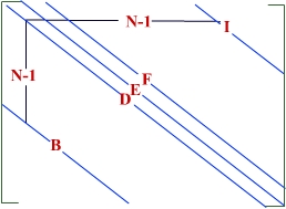
Figure 6.5.3 Structure of L for Poissons and Laplace's Equations.
Example 6.5.1: Consider the Poisson's equation
in the unit square with Dirichlet boundary conditions u(x,y) =0 on the boundary x=0, x=1, y=0 and y=1. Find the unknown variable u in the region 0 < x, y < 1 with step lengths in x and y directions,  =
=
 = 0.25.
Solution: The computational mesh for the given problem is
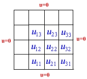
There are 9 unknown values to be obtained by solving the system (6.5.10) with i = 1, 2, 3 and j =1, 2, 3.
With A=C=1 and =
=0.25 the system (6.5.10) takes the form
for i = 1, 2, 3 and j = 1, 2, 3 ................. (6.5.11)
that is, the system (6.5.11) in matrix form Lu=G has the coefficient matrix
Gauss - Siedel solution
| u11 |
u21 |
u31 |
u12 |
u22 |
u32 |
u13 |
u23 |
u33 |
| 4.774 |
6.205 |
6.747 |
7.891 |
8.298 |
7.891 |
6.747 |
6.205 |
4.774 |