6.6 Hyperbolic Equations
If the second order partial differential equations are classified with the help of its characteristics, an hyperbolic equation in a two-dimensional domain will have two real characteristics whereas a parabolic has one and elliptic equation has only complex characteristics. Since at any point of the domain these two characteristics are orthogonal in direction (one is called the left characteristic and the other is called the right characteristic) these curves can be used as a mesh to find solutions of hyperbolic equations and the scheme is called method of characteristics.
Since a first order partial differential equation has also a real characteristic exist at each point of the domain similar to second order hyperbolic equation, these equations are also called as hyperbolic equations. Hence first order PDE also comes under hyperbolic type and is important to understand the method of characteristics and application of finite differnce methods to these first order equations.
In the present section the numerical methods and the method of
characteristics to first order PDE is considered first and then
these methods are extended to second order PDE in the consequent
sections.
Consider the first order PDE

.................
(6.6.1)
where a, b and c are
functions of x, y and u but not of  and
and
 so that the equation
(6.6.1) is called quasi-linear. (It is linear if they are functions of x and
y alone and are non-linear if they are also functions of
  and
and
 ).
).
An equivalent form of (6.6.1) is

.................
(6.6.2)
where p= and q=
 .
.
If we consider a curve C in the xy-plane other
than the curve  at which the initial conditions of u have been specified, then in directions tangential to C from the points on C. We have

.................
(6.6.3)
By eliminating p from (6.4.2) and (6.4.3) we get,


.................
(6.6.4)
Now if we choose the curve C such that

.................
(6.6.5)
on C then

.................
(6.6.6)
The curve C is called the characteristic curve and
along this curve we have from (6.6.5) and (6.6.6)

.................
(6.6.7)
or

.................
(6.6.8)
u can be obtained at any C by integrating
(6.6.8).
Example 6.6.1: Find the solution
u satisfying  and the initial condition.
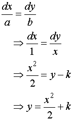
Solution: The family of characteristics
from equation (6.6.5) is
 (where k
is a constant.)
Now the values of k along the two characteristics
passing through the end points (0,0) and (0,1) of the initial curve
are k=0 and k=1 respectively. For the
characteristic through (0, yc). We have
k=yc , hence this characterisic can be
written as

The solution along this characteristic is ( from equation
(6.6.8))

gives u = 5x+A
where A
is a constant.
If u=uc at (0, yc)
then A=uc
and along the characteristics  .
We have the solution

since u is known only on the line segment  ,
the solution is also defined only in this region with bounding characteristics
 and
and  .
.
In this region the solution is unique and is not defined
outside the region  .
If the initial curve is given along any of the characteristics then
the initial values can' t be fixed arbitrarily since the solution
has to satisfy the characteristic equation
 .
.
However the initial curve differs from any characteristic then
the solution along this curve can be fixed arbitrarily. Also if the initial
conditions are given along any characteristic say along  then the equation

is also a solution at any point of the domain. That is in this
case the solution is not unique at any point not on the chosen characteristic
 .
.